


Next: Imaging
Up: Single-field imaging and deconvolution
Previous: Single-field imaging and deconvolution
Contents
Index
The measurement equation of an instrument is the relationship between the
sky intensity and the measured quantities. The measurement equation for a
millimeter interferometer is to a good approximation (after calibration)
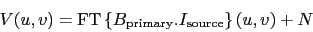 |
(4.1) |
where
 is the bi-dimensional Fourier transform of
the function
is the bi-dimensional Fourier transform of
the function  taken at the spatial frequency
  ,
,
 the sky intensity distribution,
 the primary beam of the
interferometer (i.e. a Gaussian whose FWHM is the natural resolution of the
single-dish antenna composing the interferometer),
the primary beam of the
interferometer (i.e. a Gaussian whose FWHM is the natural resolution of the
single-dish antenna composing the interferometer),  some thermal noise
and
some thermal noise
and  the calibrated visibility at the spatial frequency .
This measurement equation implies different kinds of problems.
the calibrated visibility at the spatial frequency .
This measurement equation implies different kinds of problems.
- The presence of noise leads to sensitivity problems.
- The multiplication of the sky intensity by the primary beam implies a
distortion of the information about the intensity distribution of the
source.
- The presence of the Fourier transform implies that visibilities
belongs to the Fourier space while most (radio)astronomers are used to
work in the image space. A step of imaging is thus required to go
from the
 plane to the image plane.
- Finally, the main problem implied by this measurement equation is
certainly the irregular, limited sampling of the plane because it
implies that the information about the source intensity distribution is
incomplete.
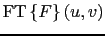
To show that deconvolution techniques are needed to overcome the incomplete
sampling of the plane, we need additional definitions
- Let's call
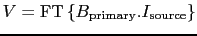 the
continuous visibility function.
the
continuous visibility function.
- The sampling function
 is defined as
-
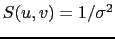 at spatial frequencies where
visibilities are measured by the interferometer.
at spatial frequencies where
visibilities are measured by the interferometer.  is the rms
noise predicted from the system temperature, antenna efficiency,
integration time and bandwidth. The sampling function thus contains
information on the relative weights of each visibility.
is the rms
noise predicted from the system temperature, antenna efficiency,
integration time and bandwidth. The sampling function thus contains
information on the relative weights of each visibility.
 elsewhere.
- We finally call
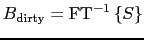 the dirty
beam.
the dirty
beam.
If we forget about the noise, we can thus rewrite the measurement equation
as
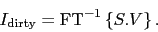 |
(4.2) |
Using the property #1 of the Fourier transform (see Appendix), we obtain
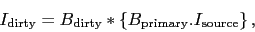 |
(4.3) |
where  is the convolution symbol. Thus, the incompleteness of the
sampling translate in the image plane as a convolution by the dirty
beam, implying the need of deconvolution. From the last equation, it is
easy to show that the dirty beam is point spread function of the
interferometer, i.e. its response at a point source. Indeed, for a point
source at the phase center,
is the convolution symbol. Thus, the incompleteness of the
sampling translate in the image plane as a convolution by the dirty
beam, implying the need of deconvolution. From the last equation, it is
easy to show that the dirty beam is point spread function of the
interferometer, i.e. its response at a point source. Indeed, for a point
source at the phase center,
 at the phase center and 0 elsewhere and the convolution with
a point source is equal to the simple product:
at the phase center and 0 elsewhere and the convolution with
a point source is equal to the simple product:
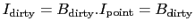 for a point source of
intensity
for a point source of
intensity
 Jy.
Jy.
Next: Imaging
Up: Single-field imaging and deconvolution
Previous: Single-field imaging and deconvolution
Contents
Index
Gildas manager
2014-07-01