


Next: Deconvolution (MOSAIC, HOGBOM, CLARK
Up: Mosaicing
Previous: Observations and processing
Contents
Index
Imaging (UV_MAP and RUN MAKE_MOSAIC)
When combining together (dirty or clean) images, it is important to correct
the primary beam attenuation to avoid modulation of the signal in the
combined image. If we forget for the moment the dirty beam convolution, the
images associated to each fields are noisy measurement of the same quantity
(the sky brightness distribution) weighted by the primary beam. The best
estimation of the measured quantity is thus given by the least mean square
formula
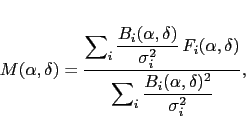 |
(5.3) |
where
 is the brightness of the dirty/cleaned mosaic
image in the direction
is the brightness of the dirty/cleaned mosaic
image in the direction
 ,
,  are the response functions
of the primary antenna beams in the tracking direction of field
are the response functions
of the primary antenna beams in the tracking direction of field  ,
,  are the brightness distributions of the individual dirty/cleaned maps, and
 are the corresponding noise values. As may be seen on this
equation, the intensity distribution of the mosaic is corrected for primary
beam attenuation. This implies that noise is inhomogeneous. Indeed, if
are the corresponding noise values. As may be seen on this
equation, the intensity distribution of the mosaic is corrected for primary
beam attenuation. This implies that noise is inhomogeneous. Indeed, if
 is the noise distribution and
 is
its standard deviation in the direction
is
its standard deviation in the direction
 , we have
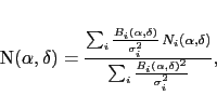 |
(5.4) |
and
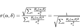 |
(5.5) |
Not only, the noise strongly increases near the edges of the mosaic
field-of-view. But also, the center of each field is contaminated by
increased noise level coming from the external regions of the neighboring
fields. Indeed, the noise corrected for the primary beam attenuation is
largely increasing where the primary beam is going to zero. To limit these
effects, both the primary beams used in the above formula and the resulting
mosaic are truncated.
Next: Deconvolution (MOSAIC, HOGBOM, CLARK
Up: Mosaicing
Previous: Observations and processing
Contents
Index
Gildas manager
2014-07-01