


Next: Attenuator
Up: Reduced Chopper Calibration
Previous: Reduced Chopper Calibration
Contents
This scheme has been implemented on Plateau de Bure, where the dynamic
range of the detectors is relatively small (only 2 between optimum
sensitivity and saturation). The only change from the standard equations
presented before is the introduction of the ``beam filling factor'' or
``calibration efficiency''  in the output on the chopper (from Eq.
(1-2))
in the output on the chopper (from Eq.
(1-2))
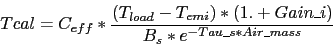
 |
(17) |
Algebra similar to that already exposed yields
 |
(18) |
just correcting  by an additional scaling factor.
In TREC mode, the sky emission is derived by
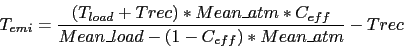 |
(19) |
and in AUTO mode, the receiver temperature may be derived by
 |
(20) |
Gildas manager
2014-07-01