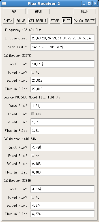
When clicking on FLUX (in the CLIC menu; Fig. ![[*]](crossref.png) ) a
widget similar to the one shown in Fig. is
opened. The flux calibration is an iterative process in which the
known flux of one or more calibrators is fixed to determine the
efficiencies (Jy/K) of the antennas, which are then used to estimate
the flux of the other calibrators. When a flux is fixed, SOLVE
derives efficiencies and fluxes. GET RESULT, STORE, and
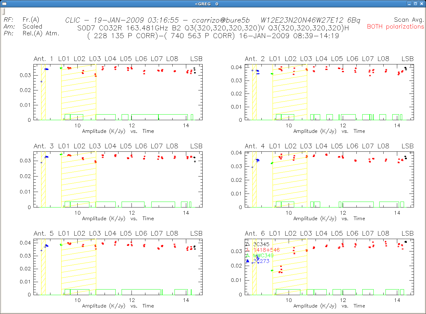
PLOT store the solved flux densities and plot the amplitudes
scaled by the derived fluxes (in K/Jy). These scaled amplitudes
correspond to the inverse of the antenna efficiencies, that, in an
ideal project, should remain constant and equal to their nominal
values.
) a
widget similar to the one shown in Fig. is
opened. The flux calibration is an iterative process in which the
known flux of one or more calibrators is fixed to determine the
efficiencies (Jy/K) of the antennas, which are then used to estimate
the flux of the other calibrators. When a flux is fixed, SOLVE
derives efficiencies and fluxes. GET RESULT, STORE, and
PLOT store the solved flux densities and plot the amplitudes
scaled by the derived fluxes (in K/Jy). These scaled amplitudes
correspond to the inverse of the antenna efficiencies, that, in an
ideal project, should remain constant and equal to their nominal
values.
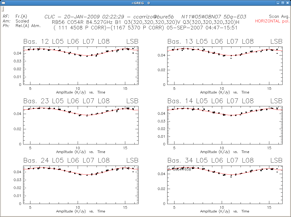
The amplitudes obtained for a calibrator often vary along the track
due to effects of a changing atmosphere or instrumental
problems. Antenna efficiencies should be estimated by considering the
best data ranges. Observational glitches, data obtained with bad
pointings or focus measurements, or limited intervals of bad data
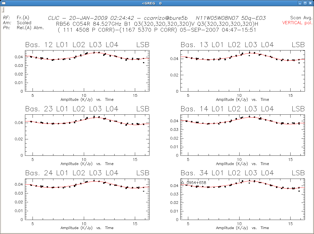
should not be considered. If for an observed polarization amplitude
oscillations on a 24 hour scale are observed, this is often an
indication of that the emission is polarized. Having H and V
polarizations is needed to confirm the presence of polarized
emission. (The degree of polarization of the PdB phase calibrators is
evaluated and archived at PdB, and so can be checked by your local
contact if needed.) Anyway, there is nothing to do in the flux
calibration with respect to this. The Scan List option permits
to select the scan ranges to be considered in the calculation of
fluxes and efficiencies. After PLOT, scan numbers can be
determined by using the command ``cursor'' and clicking on the
display (an example is shown in Figure ).
All the calibrators observed during the track are shown in this
widget. Currently the main flux calibrator is MWC349, which is
observed in most of the projects; when included, a flux is proposed to
be fixed, as we can see in Fig. . Its use must be
however considered by checking the quality of the observed
correlations: i.e. correlations on MWC349 showing a big scatter in
amplitude should not be considered unless they are representative of
the track observing conditions. The other calibrators, the one used
to calibrate the RF and also the phase calibrators, can be used in
this process. Their flux may be known from other tracks observed close
in time. Note also that we monitor the flux of the brightest
calibrators. Your local contact can provide you this information, and
also an estimate of the right efficiencies with a reasonable
accuracy. For example, for a track observed in good conditions the
expected efficiencies for the different antennas should range from 20
to 25 Jy/K, from 25 to 32 Jy/K, and from 32 to 45 Jy/K for receiver
bands 1, 2, and 3 respectively. Values much larger than those expected
should be well explained by the observational conditions. Efficiencies
significantly smaller are not possible.
|
|
|
|
As mentioned in Sect. the green lines at the bottom of
the plots show, when being above zero, the regions in which the
atmospheric phase correction is applied as resulted from PhCor.
Note finally that the option CHECK, at the top of the FLUX
calibration widget (Fig. ), permits to obtain a
solution by fixing a reference calibrator and ignoring scans of
quality below a certain threshold. This may be used as a first try, a
second iteration is often needed (after storing the first one). A
solution is stored with GET RESULT and STORE, and a new
PLOT should be created accordingly.
The flux calibration is performed by averaging the amplitudes from all
the spectral units, i.e. from all the correlator
inputs8, H and V polarizations. Delays (see
Sect. and ) result in flux losses due to that
phases are frequency averaged. To correct for remaining delays you
should follow the instructions given in Sect. . Also, as
mentioned in Sect. , differences in the (frequency
averaged) phases from H and V polarization receivers introduce
amplitude losses in the flux calibration for the RF and flux
calibrators. See Sect. to correct for this effect. Note
anyway that either the presence of delays or polarization differences
are rare, since the standard PdBI observing procedures correct for
them at the very beginning of each track.
If flagged data are masked, such masks should be reset before the flux calibration. Since fluxes are solved by averaging the data of all the spectral units, we may not be able to identify problems coming from some flagged data from, for example, one of the narrows.
|